
This is the first part of a two-part article on the business cycle approach to investing. In this segment, we’ll explain the nature of the cycle and how its “seasons” can help us reduce risk and capitalize on opportunities. Part 2 is geared to understanding the characteristics of these seasons, for better risk management and superior asset allocation. Part 2 will also explain how these phases of the cycle can be identified in real time.
The heart of our investment approach focuses on business cycle associated trends for bonds, stocks and commodities and is based on two observations. First, there is a rhythm to typical business activity that has repeated continuously since the beginning of the industrial revolution over 200 years ago. Second, the ideal asset allocation and sector rotation for investment portfolios can be adjusted based on the stage of the business cycle in an effort to increase returns while reducing risks.
The calendar year transitions through four seasons. Farmers take advantage of this by sowing seeds in the spring and harvesting the resultant crops in the late summer or fall. Our allocation approach does the same thing, except that we adapt our investment policy to the prevailing “season” in the business cycle. Just as planting seeds at the wrong time of the year leads to an agricultural disaster, the emphasis of an ill-chosen asset at the wrong time can lead to a financial disaster. Rotating assets around the cycle is only possible because a typical cycle goes through a set series of chronological sequences. Identifying those economic seasons and taking advantage of their unique investment characteristics gives us an edge in asset allocation and sector placement. It’s only an “edge” because there are times, like every other investment style, when the approach disappoints. In the long run though, a consistent path to success is possible. Rather than being victimized by inevitable cyclical declines, investors can prepare for the ever-changing financial market seasons and stand to benefit from understanding the progress of the business cycle.
Before we examine the investment aspects of the business cycle, a few remarks concerning its history and characteristics are appropriate.
The Chronological Sequence
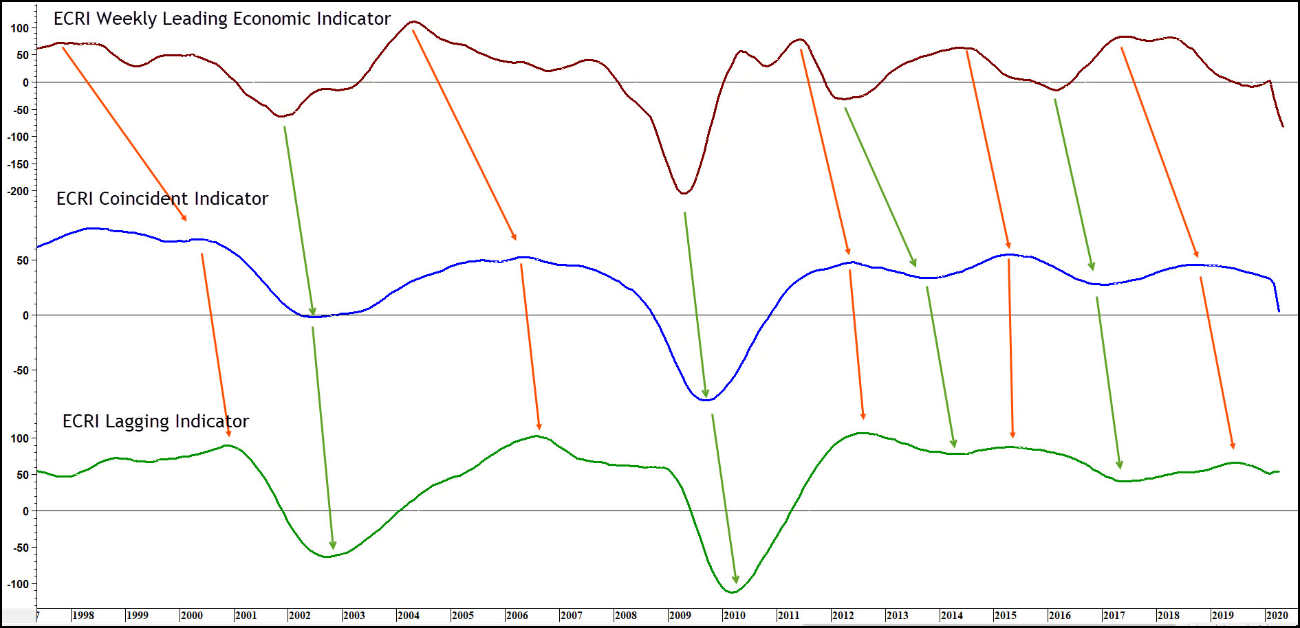
In its most simple form, a cycle can be reduced to composite indicators that reflect leading, coincident and lagging characteristics of the economy. Chart 1 features the long-term momentum for three such series, as published by the Economic Cycle Research Institute (ECRI). Note how the arrows slant to the right as they reflect the chronological sequence in the cycle. It’s important to understand that the characteristics of each one is different. This means that the leads and lags also fluctuate. So too, does the relative importance of a specific sector and its susceptibility to distortions. When we talk of “the” economy or its growth path, it’s important to understand that we’re referring to the coincident part, as opposed to the leading or lagging sectors. Also, Chart 1 greatly simplifies the turning points in the cycle, as there are literally hundreds we could list.
Every Business Cycle Experiences a Chronological Sequence
Looking at Chart 1, the cycle begins with the realization that recessionary conditions are underway. Consequently, the fed pumps in liquidity and lowers short-term interest rates. This results in a bottoming of the interest sensitive housing industry and is followed by a transition towards durable goods purchases to furnish those houses. The recovery subsequently broadens, resulting in a commodity price reversal. Eventually, rates experience a gentle rally as the demand for credit picks up. Pressure from manufacturing capacity constraints result in an eventual pick-up in capital spending. Finally, rates go up some more, thereby discouraging interest sensitive consumption such as housing and autos. At this point, sales fall at a faster pace than inventories so new orders are cut, causing the cycle to move to a recessionary phase. Eventually, this imbalance is corrected, and a new cycle is ready to begin. That was a very simplistic explanation of what can happen. In reality, recessions can be triggered by factors other than an inventory imbalance. Examples include an unexpected rapid rise in commodity prices, strains in the financial system resulting in a parabolic rise in rates for poorer quality credit instruments and so forth. One thing common to all, is a loss of confidence which causes business entities to pull back.
Chart 1 — ECRI Leading Coincident and Lagging Indicator Momentum
History of the Business Cycle
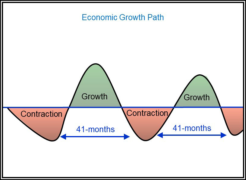
The 4-year business cycle has been with us since the beginning of the 19th century when reliable statistics first became available. It encompasses an economic expansion and contraction, as featured in Figure 1. The contractionary or recessionary phase, while not pleasant, does have a redeeming factor in that it serves as a self-correcting mechanism that cleanses the economy of previous excesses.
Figure 1 — Theoretical Business Cycle Growth Path
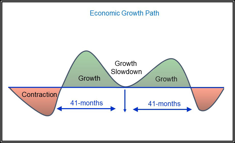
More and more over the last five decades, this corrective phase has been limited to a slowdown in the rate of growth, known as a growth recession; or just simply a slowdown. An example is shown in Figure 2. Since 1960, this plethora of slowdowns has had the effect of expanding the duration of the average time between recessions. For example, since the 1960s there have been nine recessions, which means an average between troughs of something like 80 months. However, if growth slowdowns are brought into the mix, the number of post 1960 cyclic events increases to seventeen. That translates to about 42 months, which is close to the 41-month cycle originally identified by Joseph Kitchin in the 1920s.
Slowdowns serve the same purpose as a pit stop in a car race; a step backwards in order to take several ones forward. The principal difference is that the economy actually does take a backwards step during a recession, whereas it keeps growing during the course of a slowdown, but that growth moderates and never contracts for more than a month or two.
Figure 2 — Economic Growth Path with a Slowdown

The Chronological Sequence Applies to the Financial Markets
Earlier, we established that the economy experiences a chronological sequence as the business cycle unfolds. The good news for investors is that the primary trend turning points for the financial markets, bonds, stocks and commodities, form an integral part of the chronological sequence! Their theoretical peaks and troughs have been flagged in Figure 3. For example, liquidity being thrown into the system to counteract the business contraction, allows bond prices to lead the way as they bottom during the early part of the recession. Stocks anticipate the forthcoming recovery right at the deepest part of the contraction. This is when the news is blackest and explains the apparent contradiction of stocks exploding when the economic news is so devastating. Later, when the demand and supply for commodities comes more into balance on the demand side, commodities reach their low. As the economy experiences further strength, the demand for credit grows. Consequently, its price and interest rates begin to rise, causing bond prices to peak. At the height of the recovery, players in the stock market, always looking ahead, start to anticipate the next slowdown or recession just as they had previously bottomed ahead of the recovery. Eventually, commodity prices top out as the growth path slows. Following a brief period when all three markets are in retreat, a new cycle is ready to get underway.
Figure 3 — Financial Market Business Cycle Sequence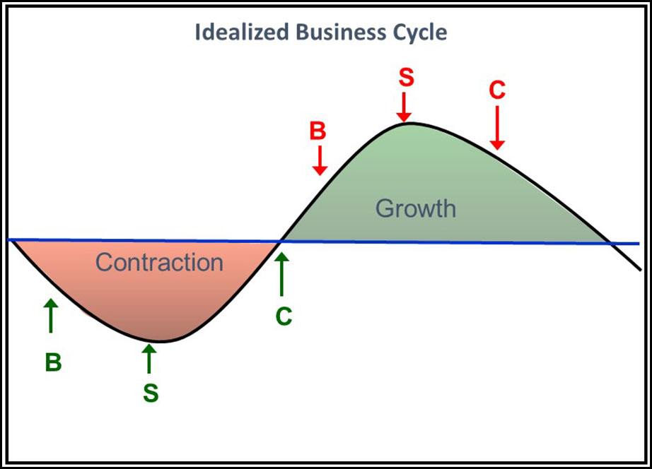
Using the Cycle as a Guide for Asset Allocation
Knowledge of the rotational nature of the markets can be used to capitalize on deflation sensitive assets in the deflationary phase of the cycle. This same knowledge can be used to downplay such assets during the cycle’s inflationary phase. That means cutting the bond allocation or shortening maturities. During the deflationary season, it’s time to play defense by emphasizing bonds and defensive equity sectors such as staples, utilities, telecom, etc. Later, when capacity tightens and commodities are running, the odds favor the purchase of earnings driven equities.
We can take this a step further by noting that there are three markets, each with two turning points. This returns six stages or investment seasons, each of which requires a different allocation make-up.
The period between 1981 and 2005 was much easier to play from the long side since the secular trend of rising prices enabled some pretty good returns to be attained. The main criticism one could lay during these two decades is that there were several instances of whipsaw activity where the Barometer kept changing its mind.
Related Article: How to Use the Business Cycle as a Proactive Risk Management Investment Tool, Part 2